Land Cover Classification
Contents
Introduction
The following guide details the processes of generating input for the Water Sensitive Cities (WSC) Scenario Tool’s extreme heat mapping module. The module is able to determine and display the spatial distribution of different land surface temperatures within a case study area – for it to do this, a land cover data file of the study area (generated from satellite imagery) is required. This text provides a step-by-step breakdown on how to prepare this item.
Initial Requirements
Before any data-preparing activities, you must have the mapping software QGIS installed on your computer. QGIS has been chosen as there is no cost associated with its adoption, and it is also available between different platforms (Windows/Mac). To obtain QGIS, navigate to the download link and follow the relevant prompts. Once these programs are installed, you are free to begin preparing data.
Raw Satellite Imagery
The first step in creating the appropriate data involves obtaining a raw satellite image of the case study area. The satellite imagery is assigned an appropriate file format and coordinate reference system via the process outlined, so that it is able to be used correctly by QGIS and the Platform.
Open QGIS. Click on ‘Plugins’ along the menu bar at the top of the QGIS display, and then select ‘Manage and Install Plugins…’. Type ‘QuickMapServices’ into the search bar, select the add-on in the whittled-down list, and click the ‘Install plugin’ button.
Click ‘Web’ on the QGIS menu bar. Hover over ‘QuickMapServices’, and then click ‘Settings’. Following the appearance of the respective dialogue box, hit the ‘More services’ button, and then press the wide ‘Get contributed pack’ button. This gives the QuickMapServices add-on access to Google Satellite.
If you possess a GIS file of the boundary of your study area, drag it into the main QGIS viewport from your file explorer.
Again, click ‘Web’ on the QGIS menu bar. Select ‘QuickMapServices’, then ‘Google’, and then click ‘Google Satellite’. QGIS should now display a satellite image of the study area and its immediate surrounds underneath the boundary layer (if you did not drag in a boundary layer into QGIS, you will need to use the cursor drag feature and the scroll wheel of your mouse to move to and zoom into your area of interest)
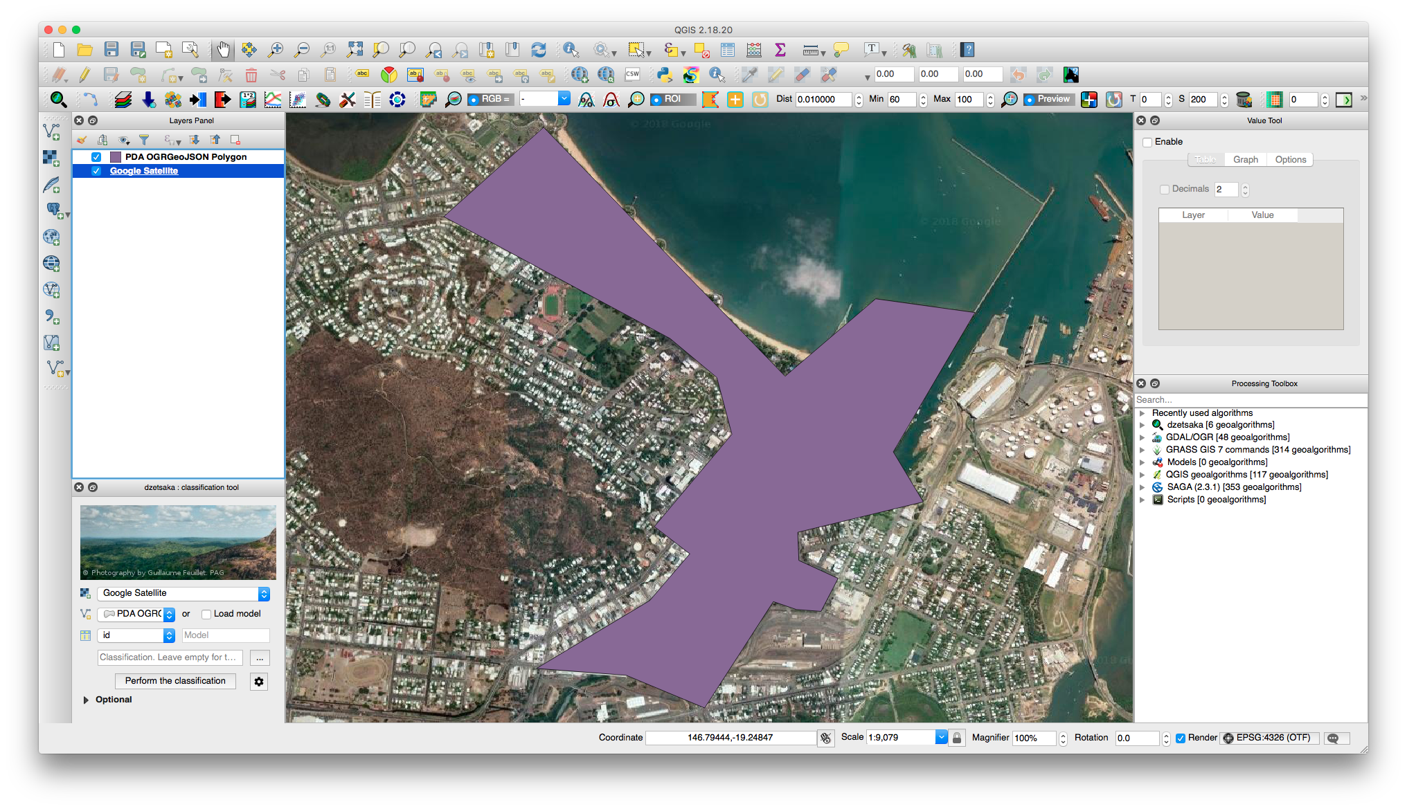
If you used a GIS boundary file, toggle its display off by clicking on the checkmarked box next to its name in the Layers Panel.
Hit ‘Project’ on the menu bar, and then click on ‘New Print Composer’. Select ‘OK’ on the dialogue box that appears. You will now be taken to the Composer window, from which you will generate a georeferenced satellite image of your study region by including what is displayed in the workspace as a map item in the current Composer viewport.
To begin what is described above, click on ‘Layout’ in the menu bar, and then hit ‘Add Map’. The cursor should now change to a crosshair – click and drag within the Composer canvas to create a boxed mirror image of the main QGIS workspace.
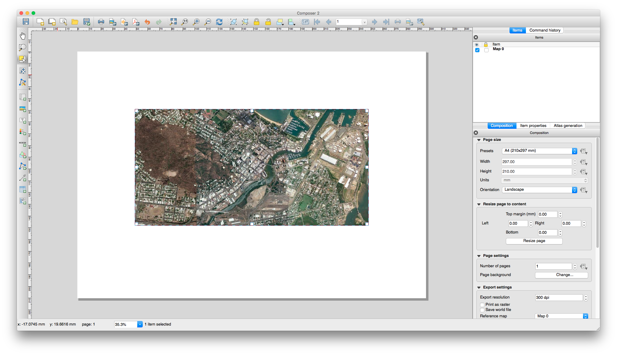
Use the small squares at the midpoints of the limits of the box to resize the image so that it completely covers the extent of the canvas (i.e. click on the small boxes and drag outward until the cursor snaps to the canvas edges).
On the panel on the right-hand side of the Composer viewport, locate and click the ‘Item properties’ button. When this is done, the forms and dropdown menus below the button should change – find and hit the button ‘Set to map canvas extent’. The workspace satellite imagery should now appear correctly, without seeming warped or containing white space (if it did so before).
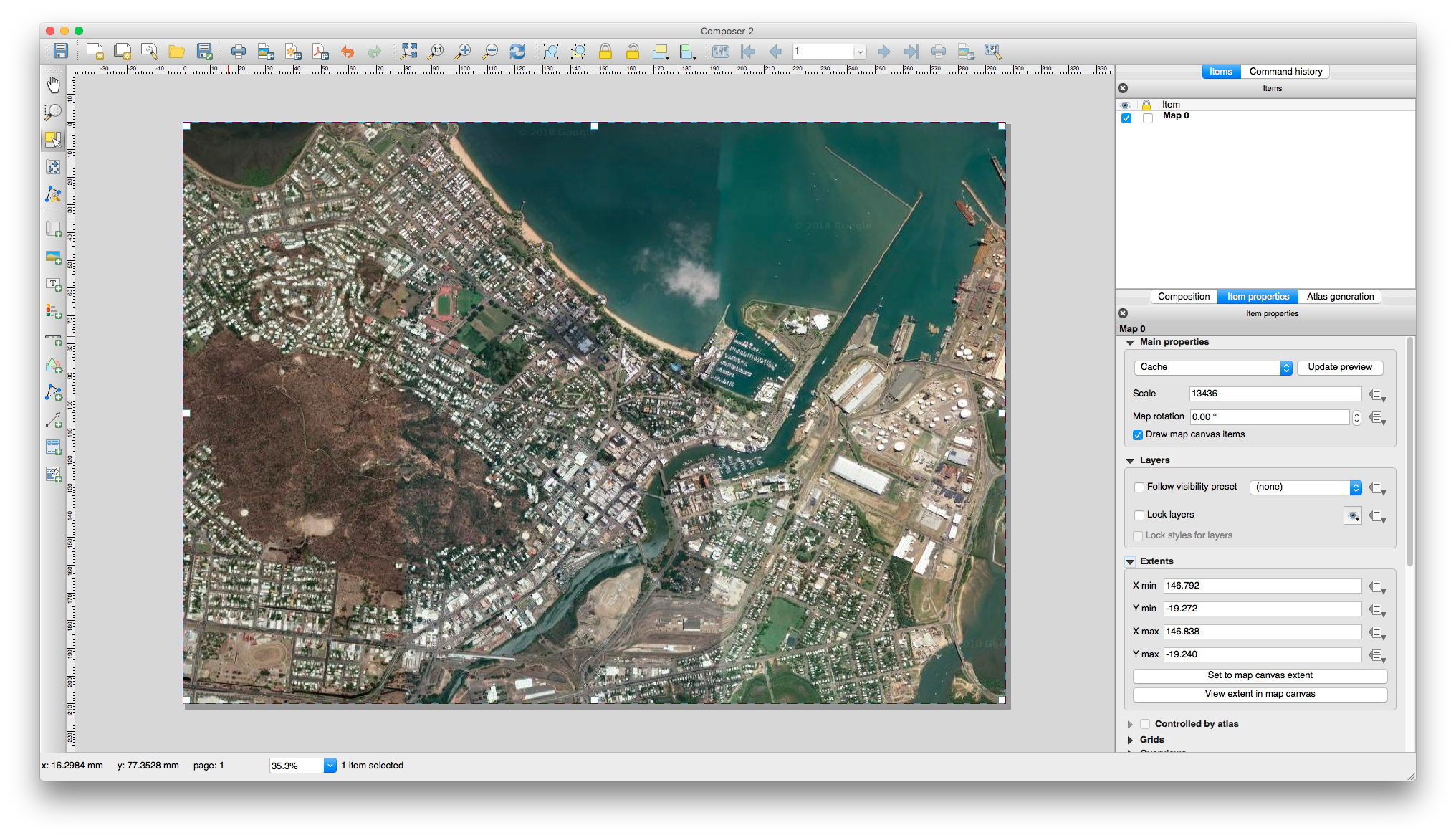
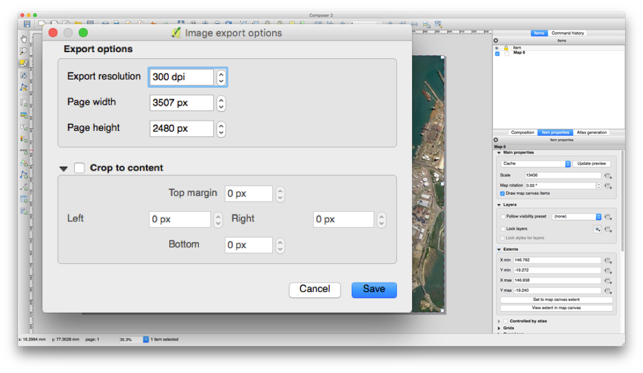
The satellite image prepared in the Composer window is now ready to be saved – click on ‘Composer’ on the menu bar, and then ‘Export as Image…’. Specify the file path for your georeferenced imagery using the dialogue box that appears, and also make sure that the file type shown in the dropdown menu is the TIFF file format. Hit ‘Save’, and another dialogue box will present itself, replacing the existing one. Use this window to adjust the level of detail picked up by the satellite imagery by increase or decreasing the ‘Export resolution’. Afterwards, hit ‘Save’, and the file will be created at the location you have designated.
Note
A good method to tell whether or not the resolution has been set high enough in the ‘Image export options’ window is by zooming in on the image (after it has been created in your computer’s file explorer) to the level at which the shape of roofs could clearly be defined using the the cursor in a given drawing program – if features appear blocky, you may required a more detailed image.
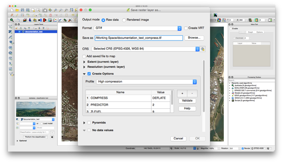
Sometimes, depending on the size and detail of your image, the file generated may be unwieldily large, and it may be in your best interests to reduce the size of the file in order to minimise storage requirements and processing speeds. To do this, first drag the TIFF file into the main QGIS workspace. Then, right-click on it in the Layers Panel window, and then hit ‘Save As…’. Give the new replacement image file a name and file path with the ‘Save as’ form , and then click on the checkbox and then the black arrow that are next to the ‘Create Options’ text – a sub-window should then appear below. Within the sub-window, click on the ‘Profile’ dropdown menu and select ‘High compression’. Hit ‘OK’ within the original section of the dialogue box, and an image much smaller in file size will be created at the desired location on your computer.
Land Cover Raster File Generation
The other process in creating suitable data input for the Platform’s extreme heat mapping module is the production of the land cover raster file; this procedure it is also the more involved. Generating a land cover raster concerns the conversion of the land surfaces communicated by the detail of the satellite imagery into categories of land cover recognised by the Platform – this is what allows the module to establish land surface temperatures.
From the menu bar at the top of the QGIS display, click on ‘Plugins’, and then ‘Manage and Install Plugins…’. In the search bar, type ‘Semi-Automatic Classification’, and then install the respective add-on by clicking on the ‘Install plugin’ button. Close the plugin window.
The SCP interface should now appear along the right side of the QGIS viewport. Within the ‘SCP input’ sub-menu, click on the dropdown button for ‘Input image’ and select the latest TIFF file you created. Then, underneath, for ‘Training input’, click on the button whose tooltip reads ‘Create a new training input’. Specify a path for the land classification training file and click ‘Save’.
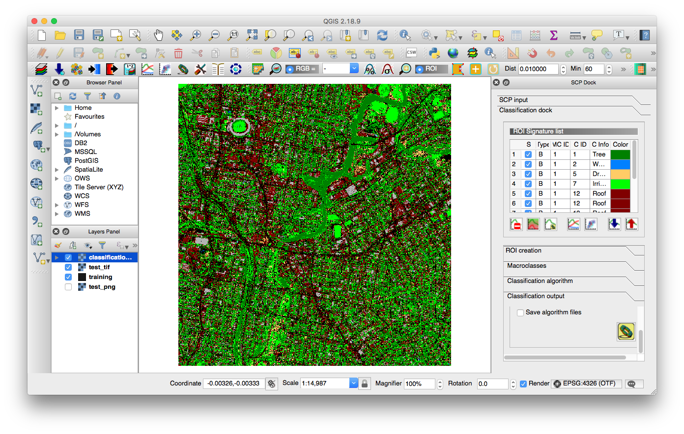
QGIS is now ready for you to specify the colour tone of the different land covers recognised by the Platform, as they appear in the satellite image. Click on the words ‘Classification dock’ in the SCP interface – this will provide you with the sub-menu enabling land cover classification.
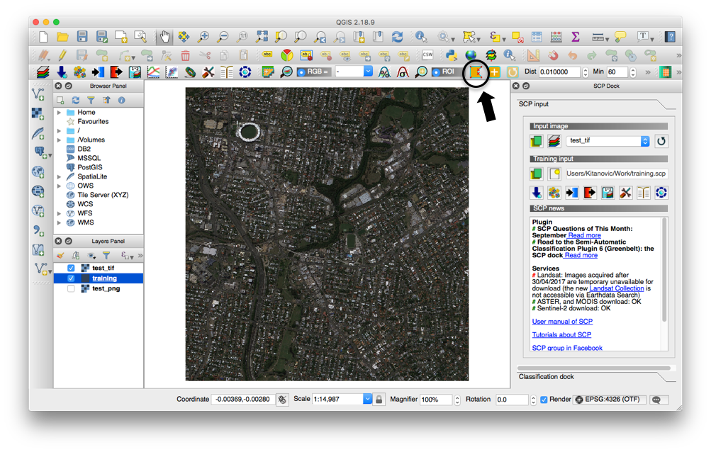
To begin the classification process, first find and click on the ROI (region of interest) polygon creation button. The button is located on one of the toolbars that appears when the Semi-Automatic Classification add-on is activated, and consists on an indiscriminate orange polygon with a light blue outline.
Once you have clicked on the button, find an area with trees within the satellite image, and generate a polygon around the trees by clicking to create vertexes (a left click signifies to the classification tool the final vertex). After doing so, under the ‘ROI creation’ heading in the SCP interface, enter ‘1’ for ‘C ID’ and ‘Tree’ for ‘C Info’ (it does not matter what you specify for ‘MC ID’ and ‘MC Info’). Click the floppy disc button to actualise the classification (ignore the warning relating to Maximum Likelihood, if it appears), and then change the colour tab for the sample within the ROI Signature list by double-clicking on it and selecting an applicable colour.
Note
It is important to consider that the sample regions must be indicative of the colour tone of the land cover as a whole, e.g. the training areas must be representative of all of a land cover’s shades. In the case of land covers whose colour can vary significantly (i.e. roofs), it is suggested that multiple training regions be created and actualised, each pertaining to one of the colour variations of the land cover, and using the same ‘C ID’ and ‘C Info’ entries. For example, in the case of the roof classification training, a polygon would be created over a house with a red roof, and then saved with a ‘C ID’ of ‘1’ and a ‘C Info’ of ‘Roof’. Then, a new polygon would be created over a house with a blue roof, and then saved with a ‘C ID’ of ‘1’ and a ‘C Info’ of ‘Roof’. The same pattern would continue until all general roof colours were accounted for.
Repeat the above step for water (C ID input ‘2’), dry grass (‘5’) irrigated grass (7’), roof (’12’), road (‘13’) and concrete (’15’) land covers, taking names (with capital first letters) as ‘C Info’ inputs (the C ID numbers stay the same for each land cover class regardless of the amount or order of samples).
Note
The land classification procedure is an iterative process, where the results of one classification inform the sampling of the next. Training regions may need to be removed, or additional regions added, in order to have the case study’s land cover properly represented. For instance, a section of road may be sampled whose color correlates to a breadth of trees, and this section of plantlife may be appearing as asphalt after the classification procedure. This training region may have to be deleted (even though it is representative of an area of road), or the trees themselves may need to be sampled (if they aren’t already) so the QGIS add-on recognises them as such. This is the nature of fine-tuning the land classification.
Once the classification training is complete, click on the ‘Classification output’ heading in the SCP interface, and then click the yellow ‘Run’ button (use the small scroll bar that appears under the heading on the right side if you cannot see it). Specify a file path and click the ‘Save’ button. The land cover raster file is now being created. Once it is complete, it will appear in the viewport and under the Layer Panel interface.
Note
Be sure to save your QGIS project, as you will not be able to access your land classification upon exiting unless it is contained within a QGIS save file.