Water Cycle Model

Introduction

The Scenario Tool functions as a planning support tool that aids in quantifying the impact of different urban form and blue/green infrastructure initiatives on an urban water catchment, and allows a variety of stakeholders to explore different development scenarios and water-sensitive strategies. As part of facilitating this, a water cycle model is incorporated within the tool’s suite of performance assessments. A water cycle model serves to detail the flow of water in and out of a specified system, with all inputs, outputs, and whatever the system retains being accounted for through the use of the principle of mass conservation. The model follows a conceptual modelling structure similar to that of current urban water management models MUSIC (eWater, 2012) and Aquacycle [Mitchell et al., 2001], with the ability to include various water-sensitive interventions within the simulation and witness how these influence both the natural and anthropogenic components of the water cycle a key advancement.

Model Summary

The Scenario Tool’s water balance model considers 2 different spatial scale:

• The lot scale, a spatial unit that represents a residential lot with a building,

a commercial or industrial lot, public spaces, roads, parks or sporting ovals. At lot scale water demand is generated, waste water produced and the hydrological processes are simulated. Further lot scale water reuse solutions such as rain water or grey water harvesting systems can be considered.

• The sub catchment scale which combines streams of water from the lots to form water supply catchments, stormwater catchments or

grey water collection catchments. The urban water cycle model supports water capture and reuse at sub catchment scale. It enables for example the capture of storm water from a precinct that is supplied into a purple pipe system for open space irrigation.

The model is implemented in CityDrain3 [Burger et al., 2016] as a conceptual node link system, routing the flows from the lot scale to the sub catchment scale on a daily time step, using 24-hour data inputs (rainfall and evapotranspiration) to produce the figures it reports. The precipitation data is sourced from the Bureau of Meteorology weather station closest to the centroid of the modelled project area, where the rainfall information from a chosen ten-year period is taken (Bureau of Meteorology, 2020). The evapotranspiration data originates from the Climate Atlas of Australia, where daily values are derived from the point potential evapotranspiration maps for each month, based again on the centroid of the project area (Bureau of Meteorology, 2001).

Lot Scale Urban Water Cycle

Lots in the Urban Water Cycle (UWC) consume and produce water, and simulate conceptually the hydrological processes. A lot in the UWC is a generic unit that can represent a residential lot with a building, a commercial or industrial lot, public spaces including roads, parks or sporting ovals.

The parameters describing a lot can found in Table 8

Table 8 Lot Scale Parameters

Name	Description
area	total area in m2
roof area	total roof area in m2
garden area	total irrigated area in m2
impervious area	impervious area exclusive of the roof area in m2
garden area	total irrigated area in m2
pervious area	calculated as area - roof area - impervious area - graden area
persons	number of people
demand profile	demand profile (see Table 10)
soil profile	soil profile (see Table 11)

The Lot scale UWC consists of three components including a water demand model that is used to estimate water consumption and waste water generation, a catchment models that aids in quantifying aspects of the hydrological cycle and a conceptual routing, storage and green infrastructure model to characterise the flows and storage behaviours at lot level detail. Fig. 17 gives an overview of the lot scale water cycle model and its streams.

Fig. 17 Schematic of how the lot scale water cycle and the default configuration of its lot scale streams.

Water demand model

The water demand model generates potable, non potable demand, and grey and black water flows as 24h timeseries data. Table 9 gives an overview of the generated streams. The demand per person is defined through the demand profile (see Table 10) and can be defined with the Water Demand Template node

Note

The water balance as defined below needs to be fulfilled potable demand + non potable demand = grey water + black water

Table 9 shows the water streams describing the lot’s urban water cycle

Table 9 Lot Scale Water Demand and Sewerage Streams

Stream	Description
potable demand	Potable demand is defined by the demand profile and multiplied with the persons on lot
non potable demand	Non-potable demand is defined by the demand profile and multiplied with the persons on lot
grey water	Grey water is defined by the demand profile and multiplied with the persons on lot
black water	Black water is defined by the demand profile and multiplied with the persons on lot

Demand profiles describe the end use per person either as a constant value per day or as time series. Typical profiles for Melbourne’s residential water consumption can be found in [Redhead et al., 2013]

The default individual residential end-use rates are denoted in Table 10 . End-uses are summed into potable or non-potable demands and multiplied by the number of relevant inhabitants to establish total indoor water demand figures for the lot. Tap, leakage and shower end-uses are taken as potable demands, and washing machine and toilet end-uses are taken as non-potable demands.

Table 10 Demand Profile

Name	Description	Default (Melbourne)
potable demand per person per day	single value or time series	77 l/p.d.
non potable demand per person per day	single value or time series	19 l/p.d.
grey water per person per day	single value or time series	19 l/p.d.
black water per person per day	single value or time series	77 l/p.d.

End-use demand rates are calculated via the water demand model, and alternative water sources are simulated through a conceptual routing and storage model for each respective intervention.

Hydrological Model

The UWC assess the hydrological water cycle at lot scale. It establishes therefore values of evapotranspiration, infiltration and runoff for the lot. The model considers pervious surfaces, irrigated pervious surfaces, roof surfaces and impervious surfaces (see Fig. 17) . For each of these surfaces runoff, infiltration and evapotranspiration are assessed as time-series in an daily time-step in m (or m3/m2). To assess the values a conceptual rainfall runoff model based on [Chiew et al., 1997] is employed (see Fig. 18). The model is widely used in Australia and used in commercial tools such as e-Water’s MUSIC [Wong et al., 2002] and AquaCycle [Mitchell et al., 2001]. The model is implemented as node in CityDrain3 ([Burger et al., 2016]).

As input the model uses 24 rainfall time series data and potential evapotransporation data from BOM. Further the soil parameters can be defined for each lot driving the hydrological model (see Table 11). The default parameters are based on MUSIC

Table 11 Soil Profile

Parameter	Default (Melbourne)
impervious threshold (m)	0.001
initial soil storage (m)	0.3
infiltration capacity (m)	0.2
infiltration exponent (-)	1
initial groundwater store (m)	0.01
daily recharge rate (-)	0.25
daily drainage rate (-)	0.05
daily deep seepage rate (-)	1
soil store capacity (m)	0.03
field capacity (m)	0.02

Following surface types and streams as 24h time series in (m) are assessed by the hydrological water cycle model:

• pervious surfaces

  • runoff (\(s_{perv}\))

  • evapotranspiration (\(e_{perv}\) )

  • deep infiltration (\(i_{perv}\) )

• irrigated pervious surfaces

  • runoff (\(s_{irr}\))

  • evapotranspiration (\(e_{irr}\))

  • deep infiltration (\(i_{irr}\))

  • outdoor demand (\(d_{out}\))

• roof surfaces

  • runoff (\(s_{roof}\))

  • evapotranspiration (\(e_{roof}\))

• impervious surfaces

  • runoff (\(s_{imp}\))

  • evapotranspiration (\(e_{imp}\))

Note that for each of the above surface types the mass balance is fulfilled. eg. \(r = s_{irr} + e_{irr} + i_{irr} + d_{out}\)

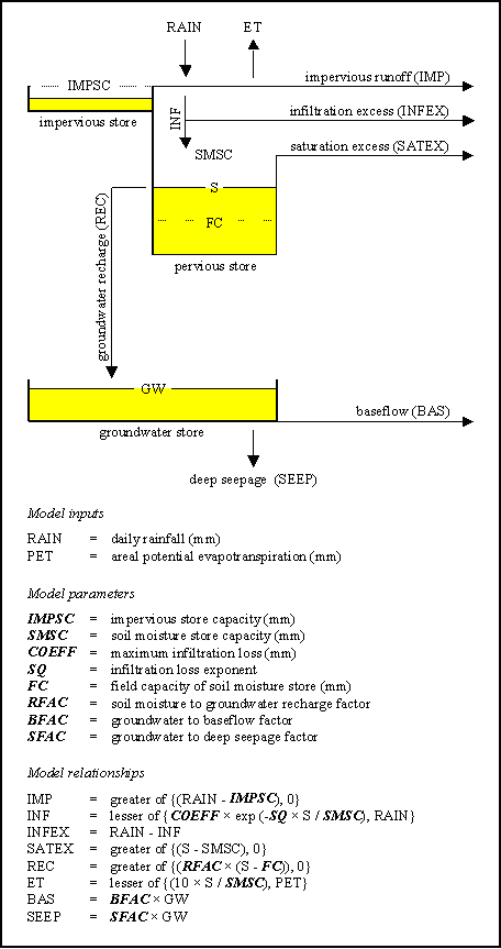
Fig. 18 Conceptual rainfall runoff model after [Chiew et al., 1997]

Table 12 Lot Scale Hydrological Streams

Stream	Description
roof runoff	\(S_{roof} = s_{roof} \cdot a_{roof}\)
impervious runoff	\(S_{imp} = s_{imp} \cdot a_{imp}\)
pervious runoff	\(S_{perv} = s_{perv} \cdot a_{perv} + s_{irr} \cdot a_{irr}\)
evapotranspiration	\(E = e_{perv} \cdot a_{perv} + e_{irr} \cdot a_{irr} + e_{roof} \cdot a_{roof} + e_{imp} \cdot a_{imp}\)
deep infiltration	\(I = i_{perv} \cdot a_{perv} + i_{irr} \cdot a_{irr}\)
outdoor demand	\(D_{out} = d_{out} \cdot a_{irr}\)

Routing

The UWC lot streams are combined to be connected to sub catchment streams. The connections are the “plumbing” of the lot and are connected to the higher level sub catchment networks. For example in the default setting the potable, non potable and out door demand stream are combined to connect to the sub catchment’s potable demand network (see Fig. 17 and Table 13). The resulting a-cyclic graph is routed with CityDrain3. Within a given timestep the flow through the nodes is in instantaneous.

Note

Note to be able to connect a sub catchment stream to the lot the connection needs to be active. For example to simulate a purple pipe a connection to non-potable demand is required. The connections can be customised with the sub catchment Lot WB Template node

Table 13 Lot Scale to Sub Catchment Stream

Stream	Sub Catchment Stream
roof runoff	stormwater
impervious runoff	stormwater
pervious runoff	stormwater
evapotranspiration	evapotranspiration
deep infiltration	deep infiltration
outdoor demand	potable demand
potable demand	potable demand
non potable demand	potable demand
grey water	sewerage
black water	sewerage

Lot Scale Storages

Lot scale storage serves to implement a representation of lot-scale water capture and reuse systems. The storage is connected to a capture stream and up to three reuse streams. The reuse streams are priorities. Water will first be provided to the stream with a higher priority until the demand is fulfilled. The overflow of the storage will be directed to the capture stream. As a result a lot scale storage will reduce the capture stream and the demand of the reuse streams. Storages can be defined with the Lot Scale Storage

The storage behaviour is implemented as a simple bucket or conceptual model and is linked into the flow network based on the defined stream configuration. [Mitchell et al., 2001]

Lot scale storages can be arranged in a cascade. Capture and reuse streams are routed through the storage cascade. This means that for example a grey water harvesting system represented as a lot scale storage can provide water for non potable and outdoor use. A rainwater harvesting tank connected in series after the grey water harvesting system will provide additional water for outdoor use.

Output

Examples of the outputs are shown below.:numref:lot_scale_inflow shows total inflow of water for all lots and Fig. 20 shows the total outflow. Note that the rainfall has been disabled in Fig. 19. The volumes reported in the user interface are the total flow after

a lot scale storage. This means, if as shown in the figures a rainwater harvesting tank (RWHT) is installed, the total inflow and outflow

will be reduced. Note, that the residual volume in the storage tank at the end of the simulation might cause a slight discrepancy when comparing the total inflow to the total outflow.

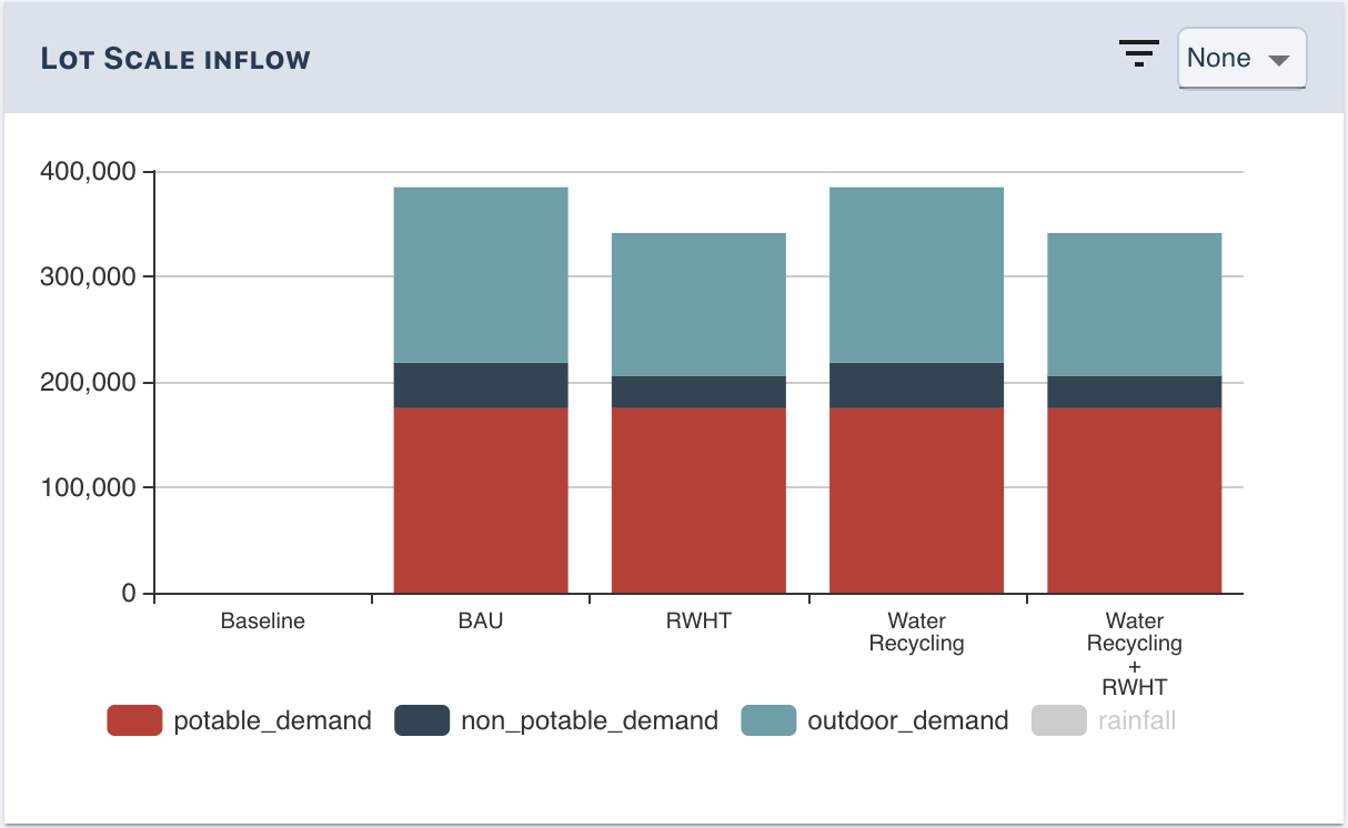
Fig. 19 Lot scale inflow

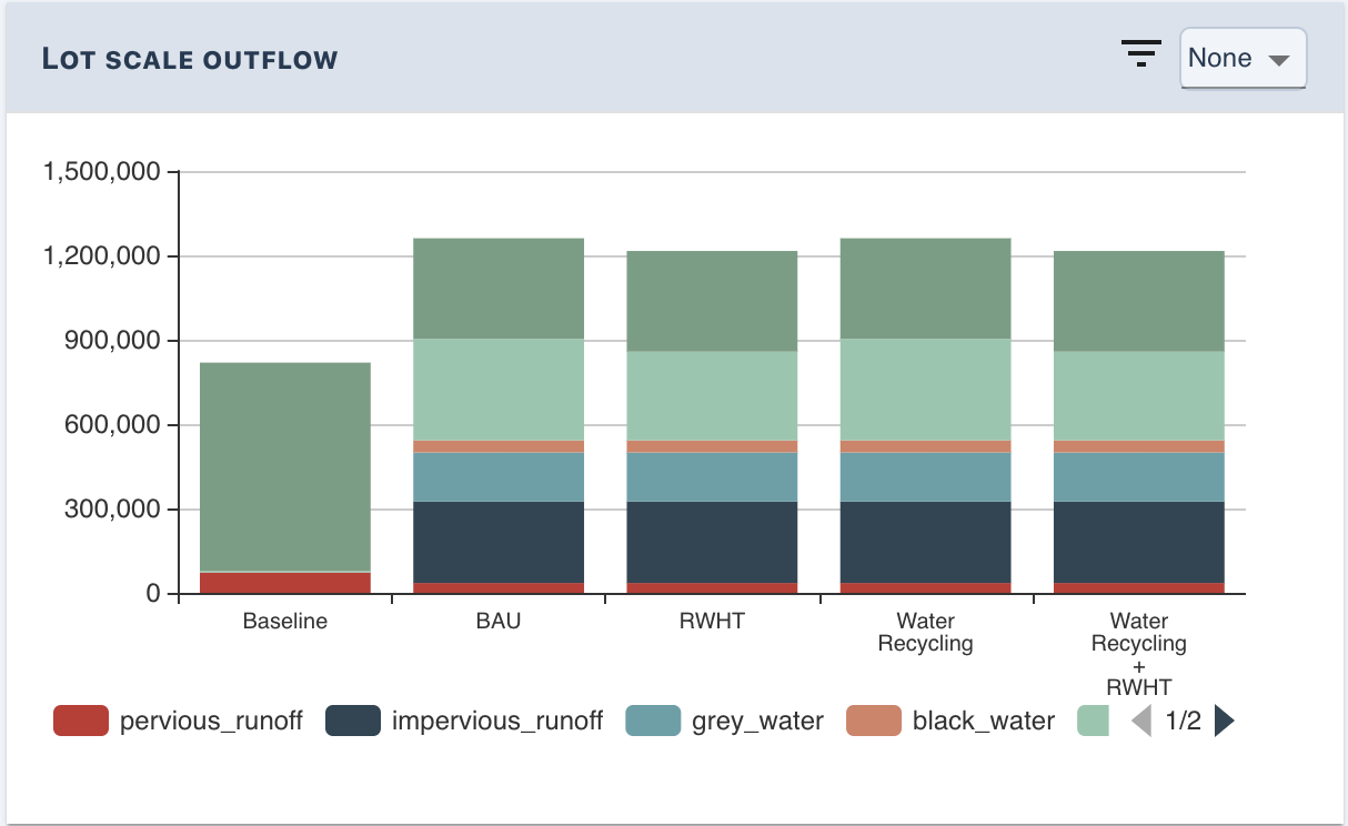
Fig. 20 Lot scale out flow

The dashboard further displays more detailed tables that report the total flow for each lot template as well as the performance of the lot scale storage (see for example Fig. 21).

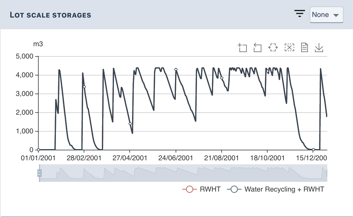
Fig. 21 Lot scale storage behaviour

Sub Catchments

The scenario tool uses sub catchments to combine streams of several lots to a catchment. For example sub catchments can be be used to represent stormwater catchments or district metering zones of the potable water network. Sub catchments combine the flow of one particular stream in a spatial region. The sub catchment regions don’t need to align. Sub catchment cen be defined using the Sub Catchment Node. Following default sub catchments defined in the scenario-tool.

• potable demand

• non potable demand

• outdoor demand

• sewerage

• grey water

• stormwater

• evapotranspiration

• deep infiltration

Fig. 22 Example routing of a sub catchment with storage

Sub Catchment Storages

Sub catchments support the implementation of storages. Sub catchment scale storages serve to implement a representation of capture and reuse system at a larger scale. For example a stormwater harvesting (see for example Fig. 22) or grey water recycling scheme. Similar to Lot scale storages sub catchment scale storages are connected to a capture stream and up to three prioritised reuse streams. Water will first be provided to the stream with a higher priority until the demand is fulfilled. The overflow of the storage will be directed to the capture stream. As a result a lot scale storage will reduce the capture stream and the demand of the reuse streams. Storages can be defined with the nodes/sub_catchment_scale_storage Node. The storage behaviour is implemented as a simple bucket or conceptual model and is linked into the flow network based on the defined stream configuration. [Mitchell et al., 2001]. Sub catchment scale storages can be arranged in a cascade. Capture and reuse streams are routed through the storage cascade.

Output

Examples of the outputs are shown below.:numref:sub_catchment_inflow shows total inflow of water for all sub catchments and Fig. 24 shows the total outflow. Note that the rainfall has been disabled in Fig. 24. The volumes reported in the user interface are the total flow after

a sub catchment scale storage. This means, if as shown in the figures a water recycling system is installed, the total inflow and outflow

will be reduced. Note, that the residual volume in the storage tank at the end of the simulation might cause a slight discrepancy when comparing the total inflow to the total outflow.

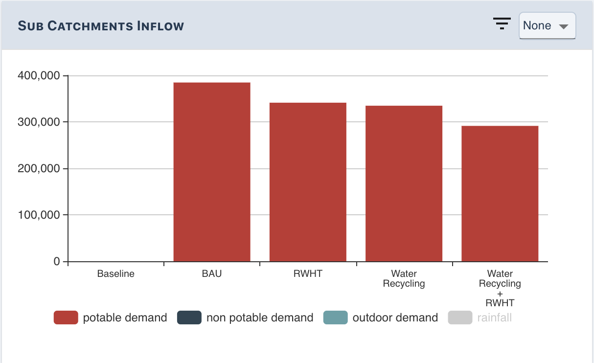
Fig. 23 Sub catchment inflow

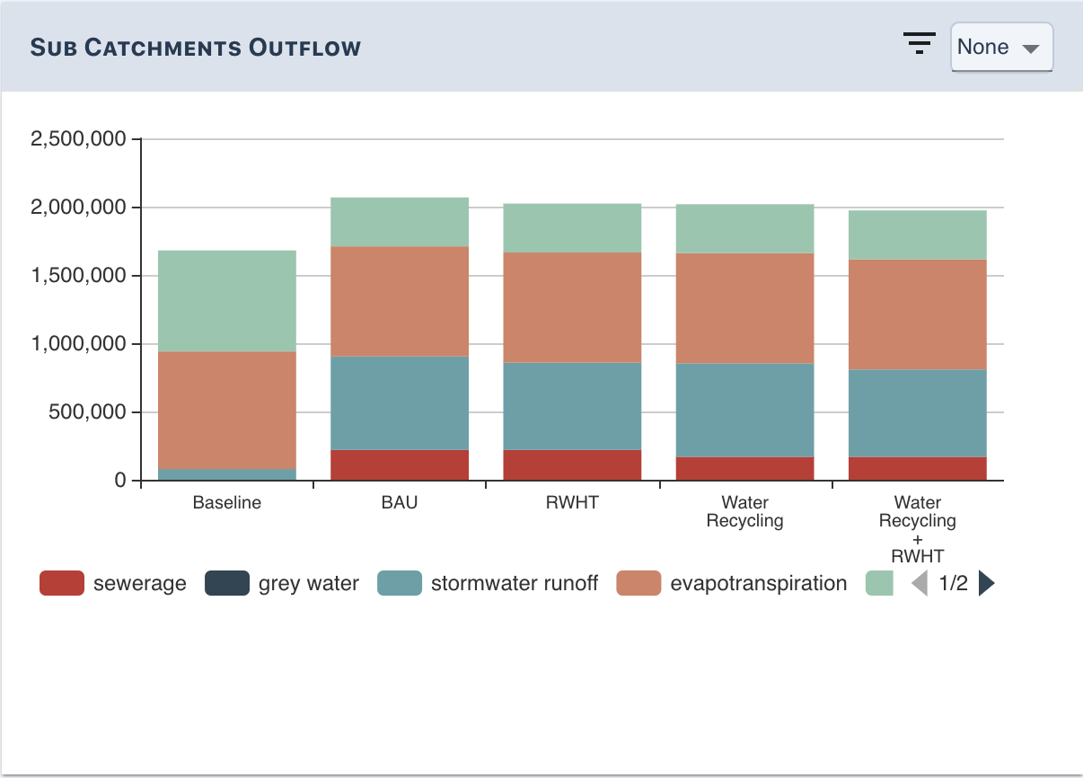
Fig. 24 Sub catchment outflow

The dashboard further displays more detailed tables that report the total flow for each sub catchment as well as the performance of the sub catchment scale storage.

Green Technologies

Considered processes:

Areas not covered by lots

Areas that are not covered by a parcel as part of a catchment will be lumped into a virtual lot. Those areas usually include transport networks or pervious areas.

The parameters are calculated as follows.

• impervious area

  • catchment area * ( average roof cover + average concrete cover + average road cover) - \(\sum\) parcel roof area + \(\sum\) parcel impervious area

• pervious area

  • catchment area - \(\sum\) parcel area - catchment area * (average water cover) - impervious area

Note that if not explicitly defined as part of a parcel green spaces and trees are considered non-irrigated.

Background

Attached a link to testing and background notebook. Test for Urban Water Cycle Model

References

Burger et al., 2016(1,2)

Burger, G., Bach, P.M., Urich, C., Leonhardt, G., Kleidorfer, M., & Rauch, W. (2016). Designing and implementing a multi-core capable integrated urban drainage modelling Toolkit:Lessons from CityDrain3. Advances in Engineering Software, 100. doi:10.1016/j.advengsoft.2016.08.004

Chiew et al., 1997(1,2)

Chiew, F., Mudgway, L., Duncan, H., & McMahon, T. (1997). Urban Stormwater Pollution. Cooperative Research Centre (CRC) for Catchment Hydrology.

Mitchell et al., 2001(1,2,3,4)

Mitchell, V.G., Mein, R.G., & McMahon, T.a. (2001). Modelling the urban water cycle. Environmental Modelling & Software, 16(7), 615–629. URL: http://linkinghub.elsevier.com/retrieve/pii/S1364815201000299, doi:10.1016/S1364-8152(01)00029-9

Redhead et al., 2013

Redhead, M., Athuraliya, A., Brown, A., Gan, K., Ghobadi, C., Jones, C., … Siriwardene, N. (2013). Melbourne residential water end uses winter 2010 / summer 2012. Smart Water Fund.

Wong et al., 2002

Wong, T. H. F., Fletcher, T. D., Duncan, H. P., Coleman, J. R., & Jenkins, G. A. (2002). A Model for Urban Stormwater Improvement: Conceptualization. Global Solutions for Urban Drainage.